Estimating the Number of Defects in Source Code
A method for estimating defects present in the source code
It would be great to know how many undiscovered defects are present in the source code. This information could be useful in:
- setting release deadlines,
- staff capacity planning,
- software quality assessment,
- evaluation of current development process.
There are several techniques for defect prediction. Most prediction techniques require historical data or data related to specific characteristics of the software project.
A well-known technique is the use of defect density per KLOC. Unfortunately defect density may vary considerably even within the same organisation, because of factors like SDLC used, architecture, software complexity, team experience etc.
Other approaches predict defects using statistical distributions like Poisson or Rayleigh. These distributions require parameters that are project specific and need to be computed from collected data (for example a measure of efficiency of the defect discovery process).
In this post I want to describe the Lincoln–Petersen method for estimating animal population sizes (also known as “mark and recapture”). This method consists of four steps:
- capture individuals of the given species (with total population
N), - mark these captured animals via a tag or a ring and then release them (
Manimals are marked), - recapture new individuals (
Canimals are recaptured in total), - find out how many have a mark (
Ranimals are marked).
The main idea behind the Lincoln-Petersen method is that the proportion of marked animals to captured animals in steps 3. and 4. is roughly equal to the proportion of all marked animals (step 2.) to the total population of the species. This can be expressed as the formula:
R/C ≈ M/NAfter rearranging the variables we can estimate the total population of animals as:
N ≈ (M*C) / RThis approach gives us only a rough estimate. If significant time passes between capture and recapture the estimate might be even more off due to animals mortality or migration.
This approach can be also used in software defect prediction. Let’s look at a concrete example.
We have a software system where we deliberately inject 15 defects into the source code. We put this system to a test and 35 defects are found out of which 6 have been injected by us. How many defects are still present in the source code? With the Lincoln-Petersen formula we get:
(15 * 35)/6 - 35 ≈ 53So most likely there are still 53 undetected defects present, 88 (53+35) defects in total. But what does most likely mean? How much more likely is it to have 88 defects in this case than let’s say 125? or 260? We would need to somehow quantify different defect count estimations (88, 125, 260, …etc.) and compare them.
The Lincoln-Petersen method gives us the most likely population value, but it does not provide any clues about the likelihood of this value being correct. Luckily statisticians came up with a clever solution for exactly this problem using the hypergeometric distribution.
This distribution computes the probability of drawing a sample of size C objects with R marked objects out of a population N objects containing M marked objects. The explanation of the distribution itself is out of scope of this post. It’s very easy to use the hypergeometric distribution in Excel via the HYPGEOM.DIST function. The Excel documentation says:
HYPGEOM.DIST returns the probability of a given number of sample successes, given the sample size, population successes, and population size.
What we can now do is iterate over different population sizes (88, 125, 260, …) and plot individual probabilities on a chart. If we do this for our example: 15 defects injected (M), 35 defects found (C) and 6 identified as the ones we injected (R) with N ranging from 0 to 321 we get the following plot:
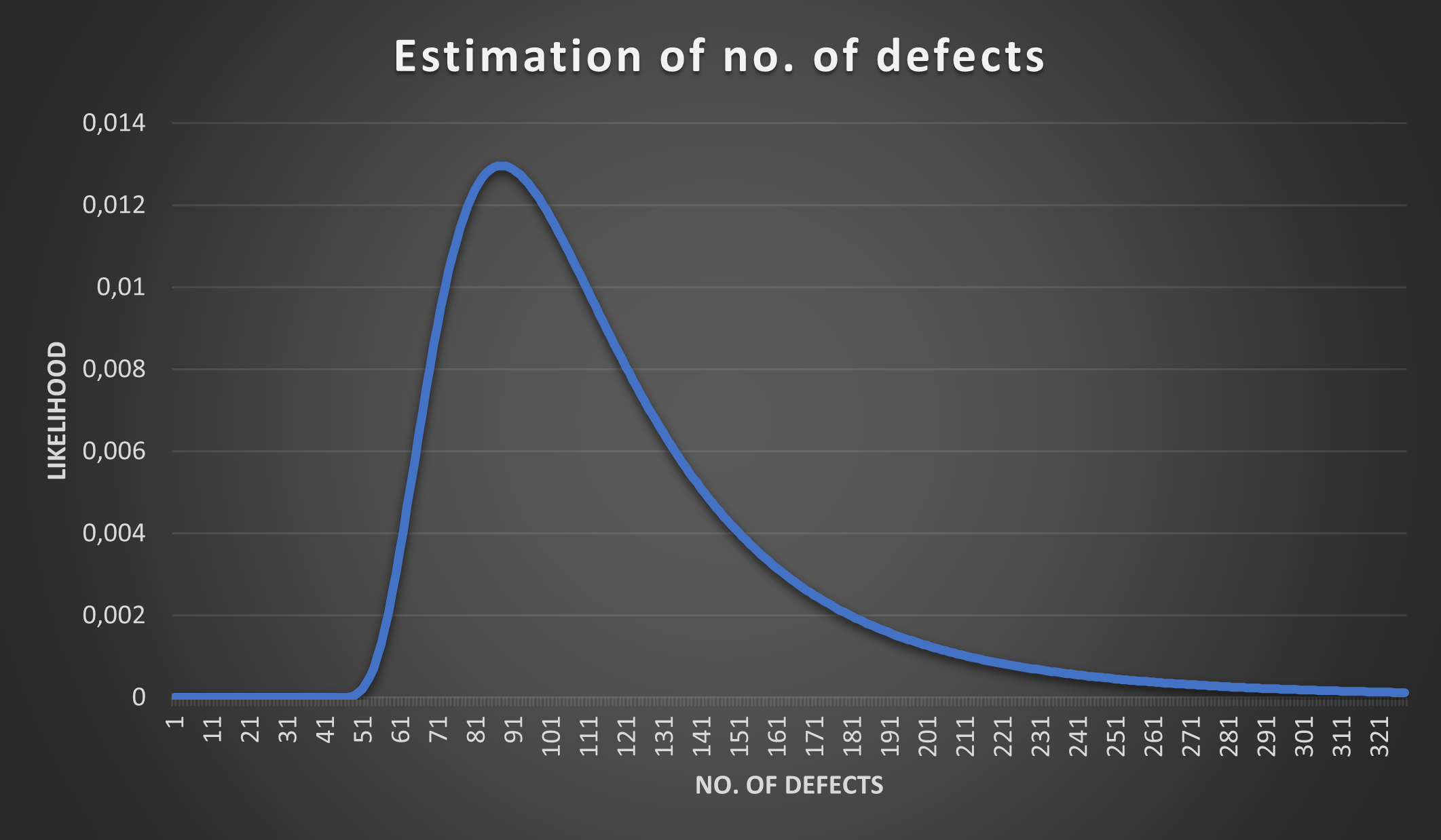
As we predicted the peak is around 88, but that does not mean that the population size (i.e. total defects) could not be 125 or 260, the chart only expresses that it’s more likely it’s around 88 than around 260.
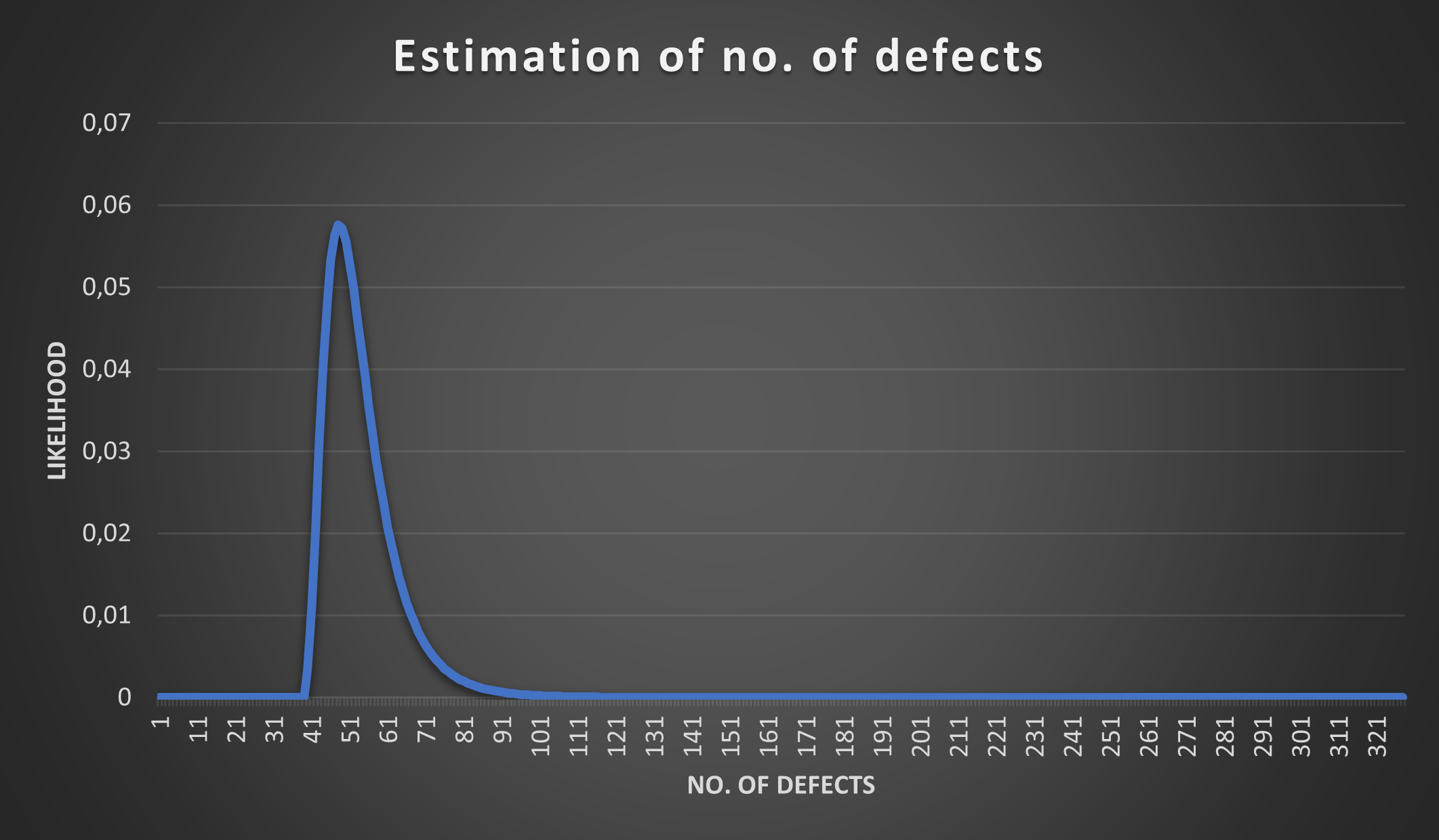
How would the probabilities change if we only found 3 injected defects in the 35 discovered defects? Let’s see what Lincoln-Petersen would predict:
(15 * 35)/3 - 35 ≈ 140So there should be around 140 undetected defects and around 175 (140+35) defects in total. Having a weak defect detection process (only 3 out of 15 injected defects detected) does not spark a lot of confidence on how many defects we actually have. Let’s plot the probabilities using R=3 with the hypergeometric distribution:
This is an interesting observation and it matches our intuition - the less injected defects we discover the higher the uncertainty about the total defect count in our source code.
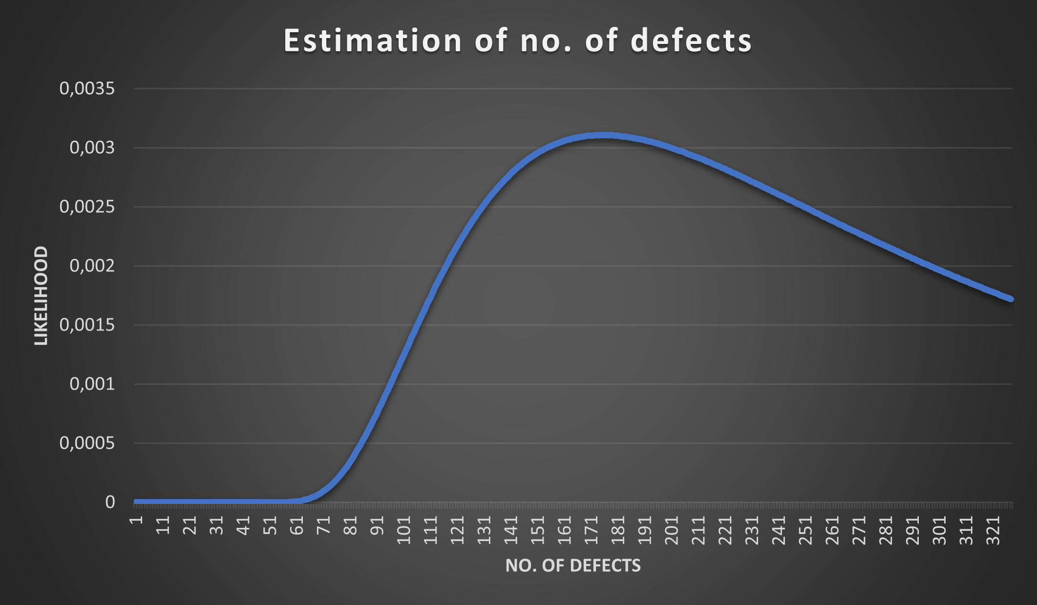
Is the opposite also true? The more injected defects we discover (among the 35) the more certain we are about the total defect count? Let’s try with R=11 (i.e. 11 out of 35 discovered defects are those that were injected):
We see what we have suspected - if we discover more injected defects the estimate narrows down. The chart however needs to be interpreted carefully.
It is likely that the total defect count is around 45 - 65, but that does not mean it can’t be 125 or 260! Although 125 and 260 have low probabilities they are not 0 (such small values are not visible on the chart, but they are non-zero). The only estimates that have 0 probability are the ones that have the value 38 or lower, why? Because if we injected 15 defects and discovered 35 (11 of which overlap with the injected) then there are at least 35 + 15 - 11 defects in the source code (i.e. at least 39 defects are present).
There are many factors impacting the quality of estimation presented above, some of them are:
- the nature of defects (there are many types of defects, we can’t lump all of them together),
- time elapsed between injecting defects and detection (the source code changes),
- process of defect detection (all defects should have equal probability of being discovered, which is usually not the case),
- …
So is this estimation useful, can it be trusted? The short answer is: I don’t know. I haven’t tried it yet and I haven’t found any scientific papers discussing this approach. If you have any experience with this approach please let me know ☺